
From Recording to Model: Real-Time Synthetic ECG Generation
From Stored ECG to Real-Time Generated ECG
In the previous post, we shared how we started building the generator using real signals taken from a database. The Raspberry Pi Pico stored the samples and replayed them. Consequently, changing the heart rate, altering the morphology, or simulating a specific condition meant preparing another recording and re-flashing it into the firmware.
In short, it acted more like a player than a generator.
Up to that point, the workflow was roughly: database → processing → samples → memory → playback.
What we were looking for was something different: parameters → mathematical model → signal → output.
This would allow us to modify signal features on the fly without having to pre-generate a new waveform. Heart rate, for example, could be a model parameter rather than a fixed property of a stored set of samples.
Searching for ways to tackle this, we came across a paper that particularly caught our attention: Cardiac Conduction Model for Generating 12 Lead ECG Signals With Realistic Heart Rate Dynamics, published in 2018 in IEEE Transactions on NanoBioscience. The paper proposes precisely a mathematical model capable of generating 12-lead ECG signals while also incorporating heart rate dynamics.
How Do We Generate an ECG from Equations?
The model represents different parts of the cardiac conduction system using dynamical oscillators. In particular, it uses three main nodes — SA, AV, and His-Purkinje — modeled with modified Van der Pol oscillators, coupled via time delays.
In addition, four other oscillators based on the FitzHugh–Nagumo model represent the primary components we recognize in an ECG: the P wave, the Ta wave, the QRS complex, and the T wave.
The final signal is constructed by combining these components. In its basic form, the model uses:
ECG = z0 + z1 − z2 + z3 + z4
and, to represent different leads, it introduces specific weights for each component:
ECG = z0 + α1z1 − α2z2 + α3z3 + α4z4
The coefficients α1 through α4 are not arbitrary: they were obtained through a fitting procedure using real ECG recordings. In much less mathematical terms: each component contributes a piece of the signal, and depending on the lead, that contribution changes.
To bring the model to the microcontroller, we implemented (and when I say implemented, I mean us together with a plethora of LLMs 😅) the equations in C and used fourth-order Runge-Kutta (RK4) numerical integration, operating at a sampling rate of 2000 Hz.
One of the aspects of the model that interested us most was the ability to work with a heart rate that wasn’t strictly constant. The paper introduces heart rate variability through an RR interval variability model, with components around 0.1 Hz and 0.25 Hz associated with low- and high-frequency bands — Mayer waves and respiratory sinus arrhythmia.
In the original implementation from the paper, this is constructed using a spectral signal and an inverse Fourier transform to obtain the RR tachogram.
We made a simpler adaptation for the Pico. Instead of implementing that whole spectral pipeline, we directly used two sinusoidal modulations — one at 0.1 Hz and another at 0.25 Hz — combined with weights of 60% and 40%.
This is not identical to what the article proposes. And we prefer to be upfront about it, because in these projects, claiming “we implemented the paper” when in reality we made an adaptation can be quite misleading.
Still, for our goal it was a great starting point. The key takeaway was that heart rate was no longer merely a static property of stored data: it could now be part of the dynamic behavior of the model.
The reference paper generates the 12 standard ECG leads and adjusts the corresponding coefficients for each of them. Our implementation, on the other hand, is built around the hardware we had already developed. We directly generate eight outputs: I, II, and V1 through V6. Leads III, aVR, aVL, and aVF are subsequently derived from the limb electrode signals.
At that stage, we had achieved something quite meaningful for us: generating an ECG through a mathematical model and altering its behavior without relying on a pre-recorded signal.
However, we still needed to see if the model was good for anything beyond generating normal sinus rhythm at a variable rate.
The paper included, among its examples, a simulation of Wellens type 1 ischemia, which features characteristic morphological changes, especially across precordial leads.
That opened up another possibility. Instead of just thinking in terms of “heart rate”, we started thinking in terms of selectable clinical conditions directly on the device. That led to several presets: normal sinus rhythm, sinus bradycardia, sinus tachycardia, SA-AV block, AV-HP block, and Wellens syndrome.
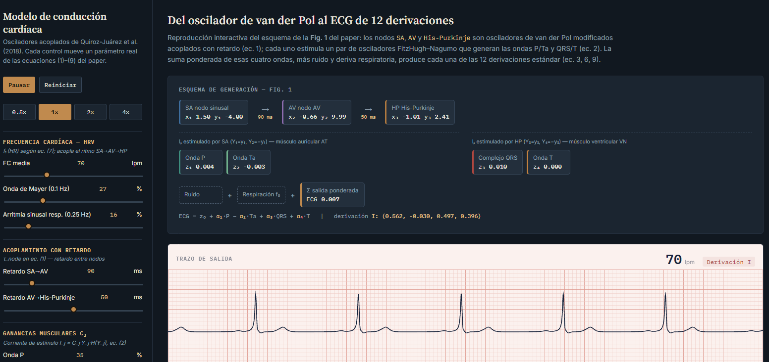
Before diving into hardware captures, here is an implementation of the same model running right in the browser, in JavaScript instead of C, but using the exact same equations and parameters we ended up running on the Pico:
Cardiac Conduction Model Simulator
It features the same presets as the firmware, all 12 leads displayed simultaneously, and live controls for adjusting heart rate, variability, and noise. It does not replace the physical generator, but it helps visualize where each wave comes from before looking at an oscilloscope, and allows anyone to experiment with the model without needing the hardware in hand.
Watching the Signal Leave the Board
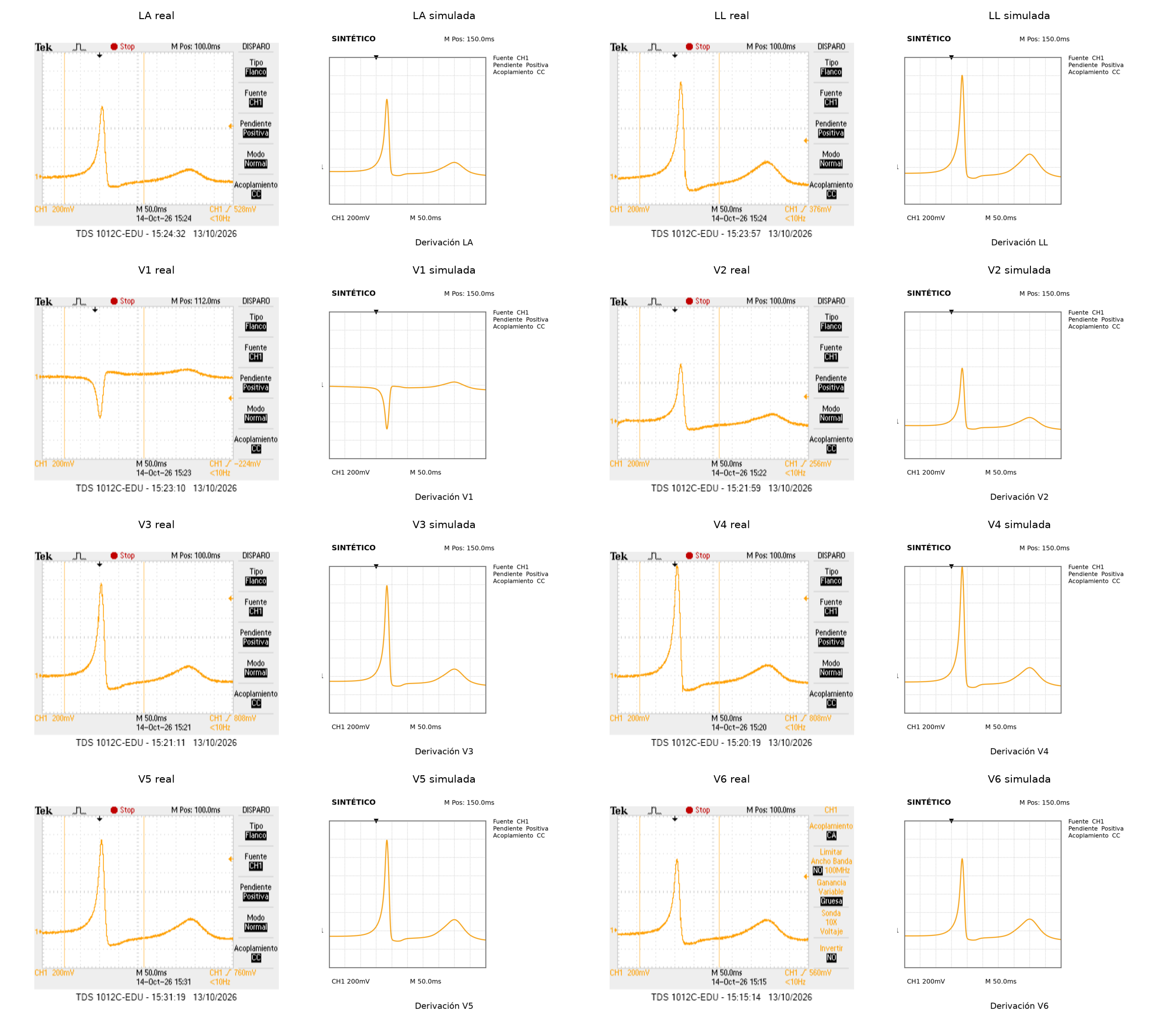
Having the model behave nicely in simulation is one thing; verifying the analog signal at the device’s output is another. For this test, we used the same filtering and conditioning hardware described in the previous post.
With the oscilloscope connected to the output of the low-pass filter, we were able to directly compare what the model predicted against what we were actually delivering.
A Control Panel to Stop Working in the Dark
As we shared in the previous post, we developed a Python application that communicates with the Raspberry Pi Pico over USB and lets us control the generator from the computer. For this phase, we expanded its controls to interface with the new model.
From the GUI, we can select the model and cardiac rhythm, adjust parameters like amplitude, component weights, and inter-nodal delays, as well as toggle heart rate variability on or off.
The most helpful feature during testing, however, was real-time signal visualization: the application streams the data generated by the Pico and plots it across leads simultaneously, allowing us to tweak a parameter and inspect almost instantaneously how the waveform changes.
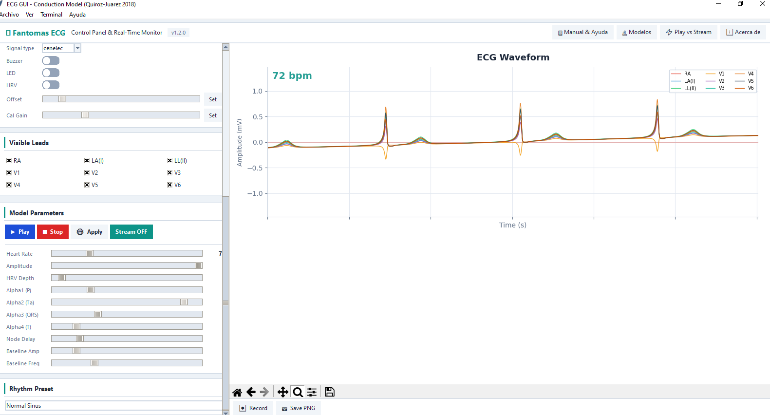
This helped us stop flying blind — relying solely on code inspection or an oscilloscope trace — and gave us a comprehensive control panel to experiment with the model and understand how each parameter adjustment impacts the ECG.
Output Calibration
We also needed tighter control over the output signal amplitude. Initially, we roughly tuned PWM values to achieve signals in the millivolt range. While the GUI displayed the waveforms, the plotted amplitude did not necessarily reflect the true analog amplitude.
To improve that estimation, we introduced a calibration routine: the Pico generates a sine wave and measures its response through one of its ADC channels.
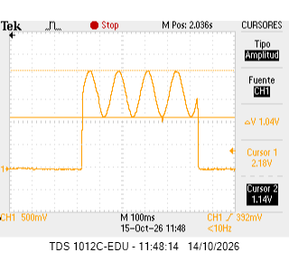
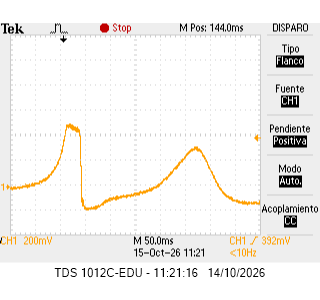
With that reading, we can map digital values to the observed amplitude and tune the output gain. Once calibrated, the GUI also indicates when clipping occurs if a requested amplitude exceeds the op-amp output range and drives it into saturation.
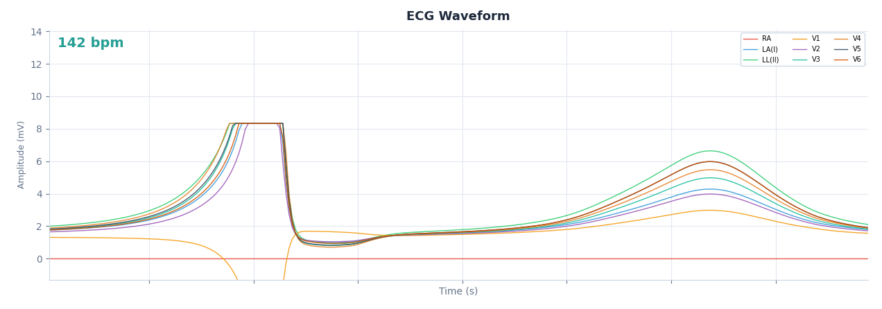
We verified this clipping behavior with the oscilloscope on output V6, where the saturation of the waveform is clearly visible:
The calibration procedure was also backported to the previous firmware, and the hardware repository was updated with the corresponding PCB changes.
From Player to Simulator
The first version of the project solved a concrete need: replaying real ECG signals to test our electrocardiograph. This second phase addressed another limitation: gaining full control over the signal.
That shift changed the core philosophy of the device. It was no longer just about hoarding a collection of ECG recordings and picking which one to play back. The premise became having a model capable of generating a signal from scratch and modulating it according to whatever we wanted to test or investigate.
Of course, challenges remained. The mathematical implementation had to live within the memory and compute limits of the microcontroller, we had to ensure the resulting signals were genuinely useful, and then there was the entire journey of analog conditioning and measurement.
But that is precisely what makes it compelling. We had transitioned from asking “which ECG can we replay?” to “which ECG can we generate?”.
In future installments, we will focus on exploring different models and assessing the signal quality they deliver.
As in the previous case, the files required for the implementation of this second version of the generator are available on GitHub, in the Laboratory repo.
